Nested Recurrent Memory

Overview

In this post, I propose a framework for multi-state Recurrent Neural Networks (RNNs). The idea: for each layer of an RNN, maintain a chain of nested memory states. Each level of the chain performs test-time regression on key-value pairs received from the level below, and each uses an identical procedure to update its own memory using those pairs. The levels fire according to an arbitrary schedule, subject only to the constraint that each level fires at a lower frequency than the one below.

At the bottom of the chain, keys and values come from the current input. Higher levels use learned, fixed-size query banks to extract values from the memory state at the next level down, then derive learned write keys corresponding to the retrieved values. This extraction apparatus is learned end-to-end. Every input token independently queries every level in the chain, producing a final output that is the sum of retrieved memories, each weighted by an input-dependent scalar. As a result, the gradient of the loss at each token cascades through the entire chain of memory consolidation — both through the memory states themselves and through the learned operators that promote information between levels. This gradient pressure allows higher levels to preserve content that proves salient downstream, protecting it from the decay and collision that would otherwise erase it at lower levels.

The framework can be instantiated for modern RNNs with vector, matrix, or function-valued memories. Its end-to-end learned nature obviates many of the memory management heuristics that define most current multi-state RNNs.

This post formalizes the framework, describes how it can be instantiated as a Nested Gated DeltaNet, and shares a naive PyTorch implementation of that instantiation. Future updates will add accompanying Triton kernels and evaluations of the trained model, to see whether the framework has value beyond its conceptual elegance.

Formal Description

In what follows, I describe only a restricted variant of the framework in which each level’s firing frequency is a multiple of the chunk size $C$ (a hyperparameter). This restriction enables efficient chunkwise parallel training (Yang et al., 2024a). Because the restricted framework coincides conceptually with its chunkwise parallel form, I describe only the latter; the recurrent form is recovered by evaluating the firing condition at the token index $t$ (using $C$ to determine chunk boundaries) and applying the per-token vector equivalents of the chunkwise matrices. Level 0 is a special case: its firing frequency is 1 in both forms, meaning it processes all $C$ tokens per chunk in the chunkwise form and updates at every token in the recurrent form. Higher levels ($\ell > 0$) fire sparsely.

Chunkwise parallel form

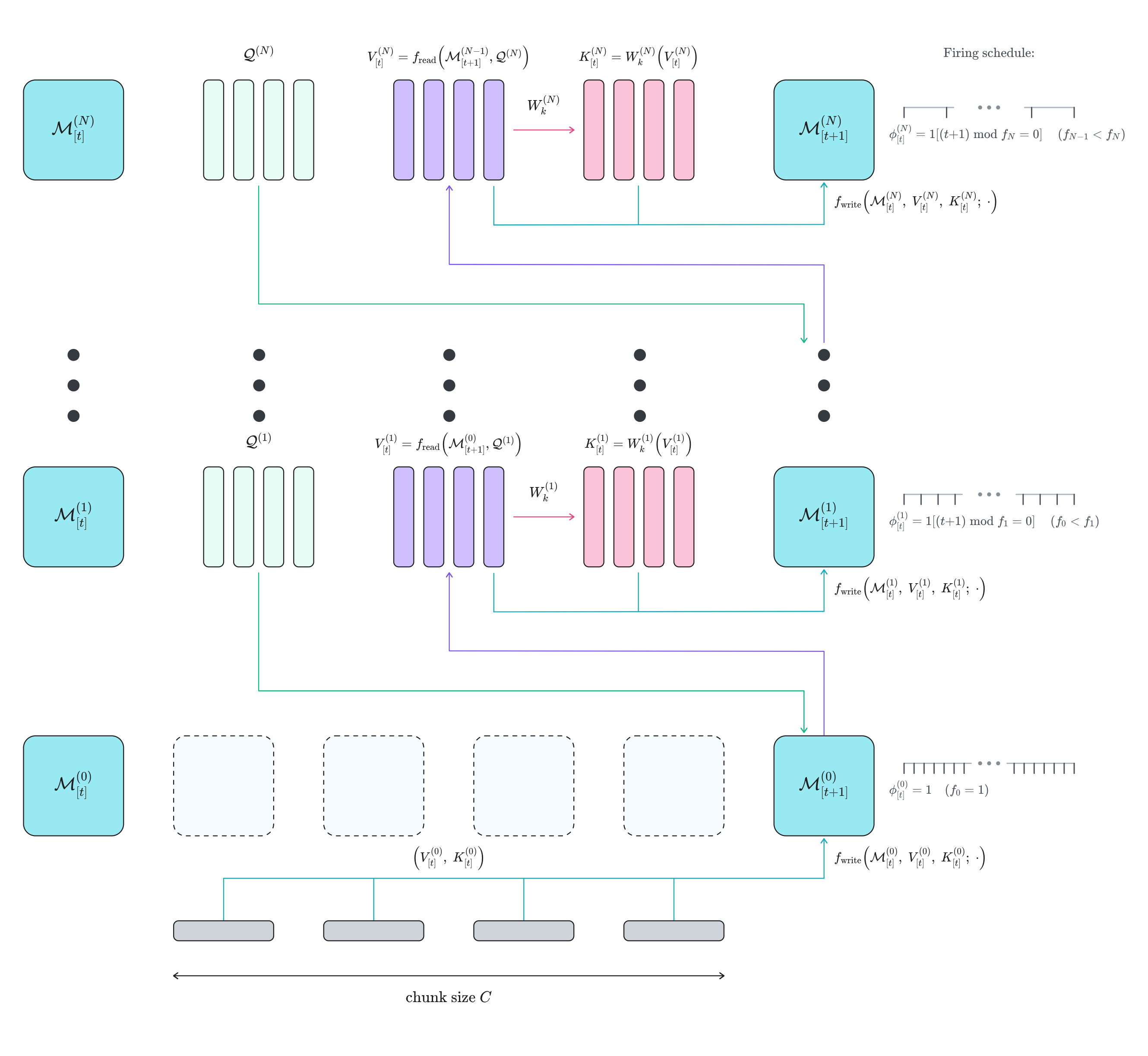
For a given layer of an RNN, I define $L$ levels. Each level $\ell$ is comprised of a memory state $\mathcal{M}^{(\ell)}$ living in some memory space $\mathfrak{M}^{(\ell)}$, and for $\ell > 0$, a fixed-size learned query bank $\mathcal{Q}^{(\ell)} \in \mathbb{R}^{n_{\ell, t} \times d_k}$. Head dimensions are elided here, and throughout, for clarity.

Let $T$ be the sequence length, $C$ the chunk size, and $N_C = T / C$ the number of chunks. Then

$$ \square_{[t]}^{(\ell)} \in \mathbb{R}^{C \times d_\square} \quad \text{where } [t] = 1:C, \quad \text{for } \square \in \{Q, K, V, R, O\} $$

defines the chunkwise matrices formed by stacking the corresponding $\square_t^{(\ell)}$ vectors over the $t$-th chunk. (Note the distinction between $Q$, the per-token read queries, and $\mathcal{Q}^{(\ell)}$, the fixed-size learned query bank at level $\ell$.)

Memory update

For each chunk $[t]$, I run every level in sequence, starting from the bottom. Each level receives a $(K_{[t]}^{(\ell)}, V_{[t]}^{(\ell)})$ pair, produced in one of two ways depending on the level.

For $\ell = 0$, the pair is derived from the input tokens by learned projections:

$$ \begin{aligned} K_{[t]}^{(0)} &= X_{[t]} W_K^{(0)} \in \mathbb{R}^{C \times d_k} \\ V_{[t]}^{(0)} &= X_{[t]} W_V^{(0)} \in \mathbb{R}^{C \times d_v} \end{aligned} $$

For $\ell > 0$, the pair is extracted from the level below using the learned query bank, then projected to form the corresponding write keys:

$$ \begin{aligned} V_{[t]}^{(\ell)} &= f_{\text{read}}\!\left(\mathcal{M}_{[t+1]}^{(\ell-1)},\, \mathcal{Q}^{(\ell)}\right) \in \mathbb{R}^{n_{\ell} \times d_v} \\ K_{[t]}^{(\ell)} &= W_K^{(\ell)}\!\left(V_{[t]}^{(\ell)}\right) \in \mathbb{R}^{n_{\ell} \times d_k}, \end{aligned} $$

where $f_{\text{read}}$ depends on the particular architectural instantiation (e.g., $\mathcal{Q}^{(\ell)} \mathcal{M}^{(\ell)}_{[t]}$ for a linear transformer, or $\mathcal{M}^{(\ell)}_{[t]}\!\left(\mathcal{Q}^{(\ell)}\right)$ for a Titans-like architecture).

With the $(K_{[t]}^{(\ell)}, V_{[t]}^{(\ell)})$ pair in hand, each level updates its memory according to the following recurrence,

$$ \mathcal{M}_{[t+1]}^{(\ell)} = \begin{cases} f_{\text{write}}\!\left(\mathcal{M}_{[t]}^{(\ell)},\, K_{[t]}^{(\ell)},\, V_{[t]}^{(\ell)};\, \cdot\right) & \text{if } \phi_{[t]}^{(\ell)} = 1 \\ \mathcal{M}_{[t]}^{(\ell)} & \text{otherwise} \end{cases}, $$

where

• $f_{\text{write}}$ again depends on the architectural instantiation (e.g., a delta rule for DeltaNet, or a SGD update on an MLP for a Titans-like architecture).
• $\cdot$ is a placeholder for additional per-level parameters (e.g., decay, gating).
• $\phi_{[t]}^{(\ell)} \in \{0, 1\}$ is the firing indicator, defined as $\phi_{[t]}^{(\ell)} = \mathbb{1}[(t+1) \bmod f_\ell = 0]$ for a per-level firing interval $f_\ell \in \mathbb{Z}^+$ (in chunks), with $f_0 = 1 < f_1 < \cdots < f_{L-1}$.

The schedule $\{f_\ell\}$ is a design choice. Common instantiations:

• Linear: $f_\ell = \ell + 1$
• Geometric: $f_\ell = C^{\ell - 1}$
• Arbitrary: any strictly increasing sequence $1 = f_0 < f_1 < \cdots < f_{L-1}$

The schedule interacts with the per-level query count $n_\ell$ in interesting ways. Slower-firing levels compress more of the sequence per event, so more extraction queries there may be warranted — e.g., $n_\ell > n_{\ell-1}$. In particular, choosing $n_\ell \propto f_\ell$ equalizes per-chunk expected compute across levels, keeping the cascade’s cost profile flat regardless of how many levels are added.

Output computation

Once each level and chunk’s memory has been updated via the usual sequential state passing procedure, the layer output is computed in parallel. It decomposes into an inter-chunk term (reading each level’s carried-over memory) and an intra-chunk term (causal self-attention within the current chunk at level 0).

Inter-chunk. For each level $\ell$, I form a per-level read query from the input tokens,

$$ Q_{[t]}^{(\ell)} = X_{[t]} W_Q^{(\ell)} \in \mathbb{R}^{C \times d_k}, $$

and read the corresponding memory from the previous chunk,

$$ R_{[t]}^{(\ell)} = f_{\text{read}}\!\left(\mathcal{M}_{[t]}^{(\ell)},\, Q_{[t]}^{(\ell)}\right) \in \mathbb{R}^{C \times d_v}. $$

The inter-chunk output combines the per-level reads via per-token, per-level mix weights:

$$ O_{[t], \text{inter}} = \sum_{\ell=0}^{L-1} \operatorname{diag}\!\left(\alpha_{[t]}^{(\ell)}\right) R_{[t]}^{(\ell)} \in \mathbb{R}^{C \times d_v}, $$

where $\alpha_{[t]}^{(\ell)} \in \mathbb{R}^{C}$ is softmaxed across $\ell$ at each token position.

Intra-chunk. Standard causal self-attention over the current chunk at level 0, reusing the level-0 read query:

$$ O_{[t], \text{intra}} = \left(Q_{[t]}^{(0)} K_{[t]}^{(0)\top} \odot M\right) V_{[t]}^{(0)} \in \mathbb{R}^{C \times d_v}, $$

where $M \in \{0, 1\}^{C \times C}$ is the usual causal mask.

Layer output.

$$ O_{[t]} = O_{[t], \text{inter}} + O_{[t], \text{intra}} \in \mathbb{R}^{C \times d_v}. $$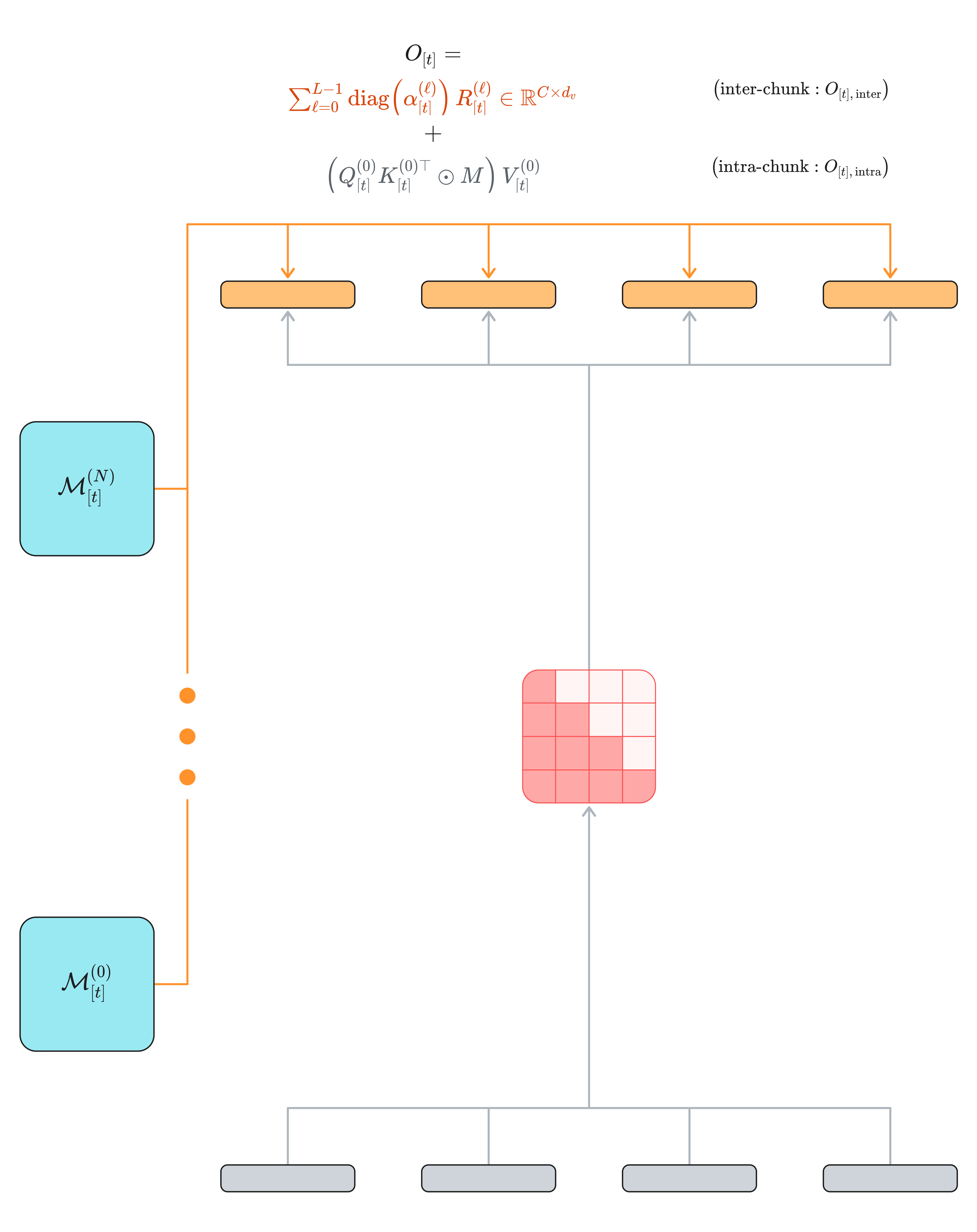

Complexity Analysis

Because higher-level firings are chunk-aligned and levels fire at strictly decreasing rates, the total work done by the cascade is a small additive term on top of the base level-0 recurrence.

Time (per layer, per forward pass).

• Level 0: Linear in sequence length. Same as the underlying single-state RNN. Denote this cost $\mathcal{O}(T \cdot c_0)$, where $c_0$ is the per-token cost of $f_{\text{write}}$ at level 0.
• Higher levels: Each level $\ell$ fires $F_\ell = T / (C \cdot f_\ell)$ times over the sequence. Each firing does $n_\ell$ extraction reads plus $n_\ell$ writes to $\mathcal{M}^{(\ell)}$, at per-event cost $c_\ell$. Total: $\sum_{\ell=1}^{L-1} F_\ell \cdot n_\ell \cdot c_\ell$.
• Reads at output: Each token performs $L$ per-level reads of cost $c_r$ each. Total: $\mathcal{O}(T \cdot L \cdot c_r)$.

Aggregate time: $\mathcal{O}\!\left(T \cdot (c_0 + L \cdot c_r) + \sum_{\ell \geq 1} \frac{T \cdot n_\ell \cdot c_\ell}{C \cdot f_\ell}\right)$, which is linear in $T$ for any bounded schedule $\{f_\ell\}$. Sub-linear firings mean the cascade contribution vanishes relative to level 0 at long sequences.

For common schedules, the firing counts $F_\ell$ decay geometrically with $\ell$ (e.g., $F_\ell = T / (C \cdot 2^{\ell-1})$ for a base-2 geometric schedule), so $\sum_{\ell \geq 1} F_\ell$ is dominated by level 1 and effectively $\mathcal{O}(T/C)$. The higher-level cascade thus contributes at most a $1/C$-fraction of the total compute — negligible for typical chunk sizes ($C = 64$ or $128$).

Space (per layer, per sequence).

• Resident state: $\sum_{\ell=0}^{L-1} |\mathfrak{M}^{(\ell)}|$, independent of $T$. Sequence length does not enter the memory footprint of the cascade itself.
• Learned parameters: Per level, extraction queries $\mathcal{Q}^{(\ell)}$ contribute $n_\ell \cdot d_k$; write projections $W_K^{(\ell)}$ contribute $\dim(V^{(\ell)}) \cdot \dim(K^{(\ell)})$; read projections contribute $d_{\text{model}} \cdot d_k$. All $\mathcal{O}(1)$ in sequence length.
• Activations (training): Per-level reads at every token must be stored for backward: $\mathcal{O}(T \cdot L \cdot d_v)$. Same $T$-scaling as the underlying RNN, multiplied by $L$.

Aggregate space: linear in $T$ during training (for the activations retained for backward), constant in $T$ at inference. The cascade adds an $L$-factor to activation memory but does not change the asymptotic scaling.

Summary. The framework preserves the linear-in-$T$ time and linear-in-$T$ (training) or constant (inference) space of the underlying RNN. Additional cost is bounded by $L$ (number of levels) and the sparse firing schedule.

Gated DeltaNet instantiation

I instantiate the framework as a nested variant of Gated DeltaNet (GDN) (Yang et al., 2024c), specifically the GDN-2 architecture (Hatamizadeh et al., 2026) at each level of the cascade. The memory space is $\mathfrak{M}^{(\ell)} = \mathbb{R}^{d_k \times d_v}$ (a state matrix per level).

Read function. For all levels,

$$ f_{\text{read}}(\mathcal{M},\, Q) = Q \mathcal{M}. $$

Write function. GDN-2’s gated delta rule with per-channel decay, erase, and write gates:

$$ f_{\text{write}}\!\left(\mathcal{M}_{[t]}^{(\ell)},\, K_{[t]}^{(\ell)},\, V_{[t]}^{(\ell)};\, \gamma_{[t]}^{(\ell)}, \beta_{[t]}^{(\ell)}, w_{[t]}^{(\ell)}\right) = \gamma_{[t]}^{(\ell)} \odot \mathcal{M}_{[t]}^{(\ell)} \left(I - \beta_{[t]}^{(\ell)} K_{[t]}^{(\ell)\top} K_{[t]}^{(\ell)}\right) + w_{[t]}^{(\ell)} \odot V_{[t]}^{(\ell)\top} K_{[t]}^{(\ell)}, $$

where

• $\gamma_{[t]}^{(\ell)} \in \mathbb{R}^{d_k}$ is a per-channel log-decay applied to the state.
• $\beta_{[t]}^{(\ell)} \in \mathbb{R}^{d_k}$ is a per-channel erase gate modulating the delta correction.
• $w_{[t]}^{(\ell)} \in \mathbb{R}^{d_v}$ is a per-channel write gate modulating the new value.

For level 0, the gates are computed per-token from the input:

$$ \gamma_{[t]}^{(0)} = \sigma\!\left(X_{[t]} W_\gamma^{(0)}\right), \quad \beta_{[t]}^{(0)} = \sigma\!\left(X_{[t]} W_\beta^{(0)}\right), \quad w_{[t]}^{(0)} = \sigma\!\left(X_{[t]} W_w^{(0)}\right). $$

For $\ell > 0$, the gates are per-firing scalars (or vectors), also learned from the input at the firing token:

$$ \gamma_{[t]}^{(\ell)} = \sigma\!\left(x_{\tau_\ell(t)} W_\gamma^{(\ell)}\right), \quad \text{etc.}, $$

where $\tau_\ell(t)$ is the token index at which level $\ell$ fires in chunk $[t]$.

Intra-chunk contribution. With GDN-2 at level 0, the intra-chunk term uses the same $(Q_{[t]}^{(0)}, K_{[t]}^{(0)}, V_{[t]}^{(0)})$ as the write path:

$$ O_{[t], \text{intra}} = \left(Q_{[t]}^{(0)} K_{[t]}^{(0)\top} \odot M\right) V_{[t]}^{(0)}. $$

Inter-chunk contribution. For the inter-chunk term, the per-token, per-level mix weights are computed as a softmax over a learned linear projection of the input:

$$ \alpha_{[t]}^{(\ell)} = \frac{\exp\!\left(X_{[t]} W_\alpha^{(\ell)}\right)}{\sum_{\ell'=0}^{L-1} \exp\!\left(X_{[t]} W_\alpha^{(\ell')}\right)} \in \mathbb{R}^C, $$

where $W_\alpha^{(\ell)} \in \mathbb{R}^{d_{\text{model}}}$ is a learned per-level projection.

Practical form. As in the original GDN-2 formulation, the recurrence is expressed with the WY representation to enable chunkwise parallelism via matrix multiplication (see Yang et al. (2024b) for derivation). The nested cascade adds a sequential dependency across levels within each chunk but leaves the level-0 hot path identical to stock GDN-2.

A naive PyTorch reference implementation of the GDN-2 instantiation is available at github.com/awehrs/nested_recurrent_memory. It includes both recurrent and chunkwise forms, verified against FLA’s stock GDN-2 at $L=1$ and mutually consistent across $L=2, 3$. Kernel implementations are coming in the next update (see Roadmap).

Related Work

Long-context studies have identified recurrent state capacity as a central limitation of linear attention models (Arora et al., 2024a; Arora et al., 2024b), motivating a growing body of work on architectures that expand or restructure recurrent memory.

Multi-state RNNs

The “multi-state RNN” framing (Oren et al., 2024) characterizes a class of architectures that maintain multiple recurrent memory states rather than compressing history into a single running state. Within this framing, prior work generally involves the checkpointing of past memory states. The schedule according to which memory states are cached can either be fixed, such as with the Fenwick tree structure in Log-Linear Attention (Guo et al., 2025) or the chunk structure of RAT (Wei et al., 2025), or proceed according to some dynamically computed heuristic, such as the “State Information Score” in Dynamic Linear Attention (Wang et al., 2026).

The size of the checkpoint cache can grow with sequence length, although not quadratically as with the KV cache of the standard transformer. For example, caches in Memory Caching (Behrouz et al., 2026) (in its constant-size segmentation variant) and RAT (Wei et al., 2025) grow linearly with sequence length. Meanwhile, Log-Linear Attention’s cache grows (sensibly enough) log-linearly with sequence length.

In some architectures, cache size is held constant by using checkpoint consolidation procedures. Dynamic Linear Attention (Wang et al., 2026), for example, merges designated memory states via a simple summation. Log-Linear Attention also uses summation, but for the purpose of promoting memory states from one position within the cache to another. With this summation design, memory consolidation is learned end-to-end solely via the loss gradient’s pressure on the memory’s structure itself, but not through its influence on a parameterized consolidation operation.¹

When computing layer output, the values retrieved by memory interrogation can be combined via a weighted sum, where input-dependent scalars act as weights (see, e.g., RAT, Log-Linear Attention, Dynamic Linear Attention); but other aggregation mechanisms exist. MARCH (Zhang et al., 2026) caches cumulative recurrent-state checkpoints as “state anchors”, each associated with a compact, content-conditioned “anchor key” used to attend across all historical anchors. Similarly, Memory Caching (in one of its instantiations) uses mean pooling of entire memory states as routing keys for cache access.

Contextualized within this line of research, the framework proposed here is a Multi-state RNN with a fixed-size memory state cache. Similar to MARCH, it routes memory access via learned key addresses, but unlike MARCH and Memory Caching, these keys address individual memories rather than entire memory checkpoints. More broadly, its consolidation and routing mechanisms are parameterized by dedicated learnable operators — extraction queries and write projections — rather than being implicit in the memory update rule itself.

Expanded-memory RNNs

Another line of work seeks to break the memory bottleneck of RNNs by increasing the size of a single recurrent state but enforcing sparse addressing thereof. This can be done through outer-product-based state expansion (Qin et al., 2024), classification-based schemes (Sparse State Expansion (Pan et al., 2025)), sparse routing à la mixture-of-experts (Du et al., 2025), spatial masking of memory addresses (Cabannes et al., 2026), or temporal masking (Bayat et al., 2026), where blocks of a fixed-size memory are progressively unlocked as context grows. None of these architectures, however, allow for dynamic, learned interactions between elements of a memory partition, as is proposed here.

Continuum Memory Systems

The framework proposed here bears a strong resemblance to the Continuum Memory System (in particular its nested and sequential variants) introduced as part of the Nested Learning paradigm and instantiated in the HOPE architecture (Behrouz et al., 2025). There, memory was consolidated across temporal scales using a stack of MLPs, which fired at frequencies decreasing in stack depth. In that architecture, the minibatch of keys and values upon which a given MLP performed test-time regression was (a) anchored with respect to size by the firing frequency of the MLP (higher-level MLPs accumulate larger “context flows” than lower ones), and (b) anchored with respect to composition by the output of the previous MLP in the stack. Here, batch examples are selected in an end-to-end learned fashion, and need not target only memory addresses in its context flow, but rather whichever addresses temporally distant exigencies deem most important to consolidate and save. Perhaps more interestingly, the minibatch size can be specified via the choice of learned query bank size for a given level. Recent work on Test-Time Training (Zhang et al., 2025) suggests that scaling the effective minibatch size at which fast-weight updates occur — from tens of tokens to thousands — substantially improves both hardware utilization and state capacity. This implies that increasing query bank size with level depth in the cascade could enable optimal batch size at all levels simultaneously.

Gist Tokens

The extraction queries at higher levels are conceptually closest to Gist Tokens (Mu et al., 2023), a small set of learned tokens trained (via a restricted attention mask that structurally forces compression) to distill a prompt into a compact activation cache reusable across downstream inputs. The mechanism is spiritually similar — a small, fixed-size set of learned probes extracts a compressed representation of a longer context, trained end-to-end — but Gist Tokens compress input context for a transformer, whereas these queries compress recurrent state for an RNN. They produce a single-level summary; I produce a hierarchical cascade of summaries.

Roadmap

This post is a v1 release. Concrete next steps, in order:

1. Forward Triton kernel for the chunkwise op. Target: parity with the naive implementation, benchmarked against stock GDN-2 to measure the cascade overhead.
2. Backward Triton kernel for the chunkwise op. Enables full training at meaningful scale.
3. Fused recurrent kernel for inference-time decoding.
4. Layer wrapper integrating the op into a standard transformer block (with the input projections, mix weights, and output projections handled).
5. Pretraining runs on a small-to-medium LM (150M–1B params) over FineWeb / SlimPajama. Compared against whatever baselines my compute budget allows — ideally stock GDN-2 and a log-linear baseline at matched parameter count.
6. MQAR / zero-shot recall evals via Zoology to isolate the cascade’s contribution to associative recall.
7. Ablations on schedule choice ($f_\ell$), query bank size ($n_\ell$), and level count ($L$).

I’ll update this post with dated results as each item lands. Code lives at github.com/awehrs/nested_recurrent_memory.

Bibliography

Arora, S., Eyuboglu, S., Timalsina, A., Johnson, I., Poli, M., Zou, J., Rudra, A., & Ré, C. (2024a). Zoology: Measuring and Improving Recall in Efficient Language Models. In International Conference on Learning Representations (ICLR 2024). arXiv preprint arXiv:2312.04927.

Arora, S., Eyuboglu, S., Zhang, M., Timalsina, A., Alberti, S., Zinsley, D., Zou, J., Rudra, A., & Ré, C. (2024b). Simple Linear Attention Language Models Balance the Recall-Throughput Tradeoff. In International Conference on Machine Learning (ICML 2024). arXiv preprint arXiv:2402.18668.

Bayat, R., Behrouz, A., Mirrokni, V., & Courville, A. (2026). Proteus: Incremental Memory Activation for Long-Context Sequence Modeling. arXiv preprint arXiv:2608.16844.

Behrouz, A., Li, Z., Deng, Y., Zhong, P., Razaviyayn, M., & Mirrokni, V. (2026). Memory Caching: RNNs with Growing Memory. arXiv preprint arXiv:2602.24281.

Behrouz, A., Razaviyayn, M., Zhong, P., & Mirrokni, V. (2025). Nested Learning: The Illusion of Deep Learning Architectures. In Advances in Neural Information Processing Systems 39 (NeurIPS 2025). arXiv preprint arXiv:2512.24695.

Cabannes, L. et al. (2026). Sparse Delta Memory: Scaling the State of Linear RNNs through Sparsity. arXiv preprint arXiv:2607.07386.

Du, J., Sun, W., Lan, D., Hu, J., & Cheng, Y. (2025). MoM: Linear Sequence Modeling with Mixture-of-Memories. arXiv preprint arXiv:2502.13685.

Guo, H., Yang, S., Goel, T., Xing, E. P., Dao, T., & Kim, Y. (2025). Log-Linear Attention. arXiv preprint arXiv:2506.04761.

Hatamizadeh, A., Choi, Y., & Kautz, J. (2026). Gated DeltaNet-2: Decoupling Erase and Write in Linear Attention. arXiv preprint arXiv:2605.22791.

Mu, J., Li, X. L., & Goodman, N. (2023). Learning to Compress Prompts with Gist Tokens. In Advances in Neural Information Processing Systems 36 (NeurIPS 2023). arXiv preprint arXiv:2304.08467.

Oren, M., Hassid, M., Yarden, N., Adi, Y., & Schwartz, R. (2024). Transformers are Multi-State RNNs. In Proceedings of the 2024 Conference on Empirical Methods in Natural Language Processing (EMNLP 2024), pp. 18724–18741. arXiv preprint arXiv:2401.06104.

Pan, Y., An, Y., Li, Z., Chou, Y., Zhu, R., Wang, X., Wang, M., Wang, J., & Li, G. (2025). Scaling Linear Attention with Sparse State Expansion. arXiv preprint arXiv:2507.16577.

Qin, Z., Yang, S., Sun, W., Shen, X., Li, D., Sun, W., & Zhong, Y. (2024). HGRN2: Gated Linear RNNs with State Expansion. arXiv preprint arXiv:2404.07904.

Wang, Y. et al. (2026). Dynamic Linear Attention. arXiv preprint arXiv:2606.10650.

Wei, X., Yadav, A., Pascanu, R., & Gulcehre, C. (2025). RAT: Bridging RNN Efficiency and Attention Accuracy via Chunk-based Sequence Modeling. arXiv preprint arXiv:2507.04416.

Yang, S., Wang, B., Shen, Y., Panda, R., & Kim, Y. (2024a). Gated Linear Attention Transformers with Hardware-Efficient Training. In Proceedings of the 41st International Conference on Machine Learning (ICML 2024). arXiv preprint arXiv:2312.06635.

Yang, S., Wang, B., Zhang, Y., Shen, Y., & Kim, Y. (2024b). Parallelizing Linear Transformers with the Delta Rule over Sequence Length. In Advances in Neural Information Processing Systems 37 (NeurIPS 2024). arXiv preprint arXiv:2406.06484.

Yang, S., Kautz, J., & Hatamizadeh, A. (2024c). Gated Delta Networks: Improving Mamba2 with Delta Rule. arXiv preprint arXiv:2412.06464. Also in ICLR 2025.

Zhang, M., Yang, K., Yu, S., Hua, E., Ding, N., Hu, X., Zhou, B., Lu, C., & Sun, Y. (2026). MARCH: Scaling Recurrent Memory with Content-Routed State Anchors. arXiv preprint arXiv:2608.12435.

Zhang, T., Bi, S., Hong, Y., Zhang, K., Luan, F., Yang, S., Sunkavalli, K., Freeman, W. T., & Tan, H. (2025). Test-Time Training Done Right. arXiv preprint arXiv:2505.23884.