General implementation
The bottom level is a stock flash-linear-attention GDN-2. Higher levels differ in four ways.
1) Promoted pairs are written simultaneously. Everything a level writes at a firing comes from one snapshot of the level below, so there’s no ordering among the pairs and no principled order to apply them in. They all act on the state as it stood before the firing. This is a different operation from level 0’s, not just a faster schedule: at level 0 the chunkwise algorithm computes what sequential application would give, whereas at higher levels, applying the pairs one after another would give a different answer. Each firing is a batched regression; level 0 is still one pair per token.
2) The retrieved values are the input, and everything else is derived from them. The query bank probes the level below and gets back values. Each value’s write key is projected from the value itself, so each piece of content picks its own address, and the erase and write gates come from the value too. This mirrors level 0, where a write is a token and its gates come from that token.
3) Decay is per firing, not per pair. Erase and write gates are per pair, a straightforward projection off each value. Decay multiplies the whole state once before anything is written, so a firing needs one decay vector, and the pairs give you many.
Collapsing many into one is the awkward part. I average the per-pair log-decays, which amounts to a geometric mean of the decays. Summing has the better justification, since it’s exactly what applying the pairs one at a time would give. But it ties a level’s horizon to its query count: promote twice as many pairs and the level forgets twice as fast. The mean decouples them and is still order-invariant, though it’s an analogy rather than something inherent in the math. And the fact that one firing spans many tokens, so a level “should” decay several times between firings, is absorbed into the learned gate.
4) Every level is read at every token. The levels aren’t a pipeline. At each token, every level is queried with its own read query, and the results are mixed with per-token weights from a softmax over levels. Level 0 writes before the read, so a token sees its own write; higher levels write after, so a firing is first visible at the next token.
\begin{algorithm}
\caption{\textsc{Nested-GDN-2}($x, L, f$)}
\begin{algorithmic}
\FOR{$\ell = 0$ \TO $L-1$}
  \STATE $\mathcal{M}^{(\ell)} \gets 0$ \COMMENT{one $d_k \times d_v$ memory per level}
\ENDFOR
\FOR{each chunk $c = 1$ \TO $N$}
  \STATE $\mathcal{M}^{(0)} \gets$ \CALL{GDN-2}{$\mathcal{M}^{(0)}, K_c, V_c, \gamma_c, \beta_c, w_c$} \COMMENT{level 0: stock GDN-2}
  \FOR{each token $t$ in chunk $c$}
    \STATE $o_t \gets \sum_{\ell} \alpha_t^{(\ell)} \, q_t^{(\ell)} \mathcal{M}^{(\ell)}$ \COMMENT{read every level, mix}
  \ENDFOR
  \FOR{$\ell = 1$ \TO $L-1$}
    \IF{$c \bmod f_\ell = 0$}
      \STATE $\mathcal{M}^{(\ell)} \gets$ \CALL{Promote}{$\mathcal{M}^{(\ell)}, \mathcal{M}^{(\ell-1)}, \ell$} \COMMENT{level $\ell$ fires}
    \ENDIF
  \ENDFOR
\ENDFOR
\RETURN $o$
\end{algorithmic}
\end{algorithm}
\begin{algorithm}
\caption{\textsc{Promote}($\mathcal{M}, \mathcal{M}_{\text{below}}, \ell$)}
\begin{algorithmic}
\STATE $V \gets \mathcal{Q}^{(\ell)} \mathcal{M}_{\text{below}}$ \COMMENT{retrieve $n_\ell$ values}
\STATE $K \gets$ \CALL{Normalize}{$W_K^{(\ell)} V$} \COMMENT{each value picks its address}
\STATE $\beta \gets \sigma\left(W_\beta^{(\ell)} V\right)$ \COMMENT{erase gate, one per pair}
\STATE $w \gets \sigma\left(W_w^{(\ell)} V\right)$ \COMMENT{write gate, one per pair}
\STATE $\gamma \gets \operatorname{mean}_{\text{pairs}}\left(-\operatorname{softplus}\left(W_\gamma^{(\ell)} V\right)\right)$ \COMMENT{decay, one per firing}
\STATE $\mathcal{M} \gets \operatorname{diag}\left(e^{\gamma}\right) \mathcal{M}$ \COMMENT{decay the whole state}
\STATE $\mathcal{M} \gets \mathcal{M} - K^{\top}(\beta \odot K)\, \mathcal{M}$ \COMMENT{erase at the new addresses}
\RETURN $\mathcal{M} + K^{\top}(w \odot V)$ \COMMENT{write every pair at once}
\end{algorithmic}
\end{algorithm}
Kernel
The bottom level uses fla’s GDN-2 kernels, with one change: its backward has to accept the gradient coming down from the level above. I vendored the fla ops to add that one extra input; the math is unchanged.
Because the upper levels write their pairs simultaneously, they skip the numerical linear algebra GDN-2 needs for its sequential intra-chunk updates. That makes their kernels much simpler, so I’ll only sketch them.
The forward has two stages:
1) Probe. Plain PyTorch: probe the level below and project out the write keys, gates and decay. It’s all dense matmuls, so cuBLAS handles it.
2) Update. A Triton kernel that scans over firings. It isn’t chunkwise in the GDN-2 sense, since there’s no intra-chunk structure. A level’s state only changes when it fires, so the kernel stores one state per firing interval rather than one per chunk.
For the backward, a wrapper combines the update’s hand-written gradients with autograd through the probe. The forward runs without a graph, so the wrapper replays the probe with gradients on and differentiates that, at the cost of one extra probe forward.
The grid is split across batch, heads and blocks of the state’s value dimension. The key dimension can’t be split, because the erase step contracts over it: every row of the state contributes to every value written.
I also considered fusing both stages into one kernel, and decided against it for two reasons.
1) Parallelism and head dimension. Deriving the write keys contracts over the value dimension, so a fused kernel can only parallelize over batch and heads. Each program would also have to hold every key and value, plus the backward’s accumulators, which live for the whole scan, and that caps how many queries fit. Moving the probe out freed enough room to double the head dimension. That matters because head dimension caps the query count: the state is a K × V matrix with at most K independent addresses, so promoting more than K pairs means the memory can’t tell them all apart.
2) Swappable promotion. The probe is a PyTorch function with a fixed signature, and its backward comes from autograd, so a new promotion scheme is just a new function. I plan to compare learned promotion against a fixed merge that carries the level below up whole at identity addresses, in the spirit of Log-Linear Attention (Guo et al., 2025). Both arms gate identically; the merge arm only gives up choosing. Being able to swap that without touching the kernel mattered.
The cost is memory traffic. The split writes the probe’s outputs to memory and reads them back, where a fused kernel would keep them on chip. The backward is worse: three of its gradients reduce over the value dimension, which is exactly the one the programs are split along, so each program writes a partial result and they’re summed afterward. As the results show, it wasn’t a deal-breaker.
Results
The comparison that matters is against a flat GDN-2 holding the same recurrent state, which for L levels means a flat model with L times as many heads.
Unless noted, every nested run doubles its query count at each level (16, 32, 64, …). The query count is
effectively the batch size of each level’s test-time regression, and doubling it gives every level the same
number of promoted pairs per training step: deeper levels fire half as often, and twice the queries makes up
for it. The count can’t exceed head_dim, so at head_dim 64 the doubling tops out at four levels; the five- and
six-level runs hold the top levels at 64.
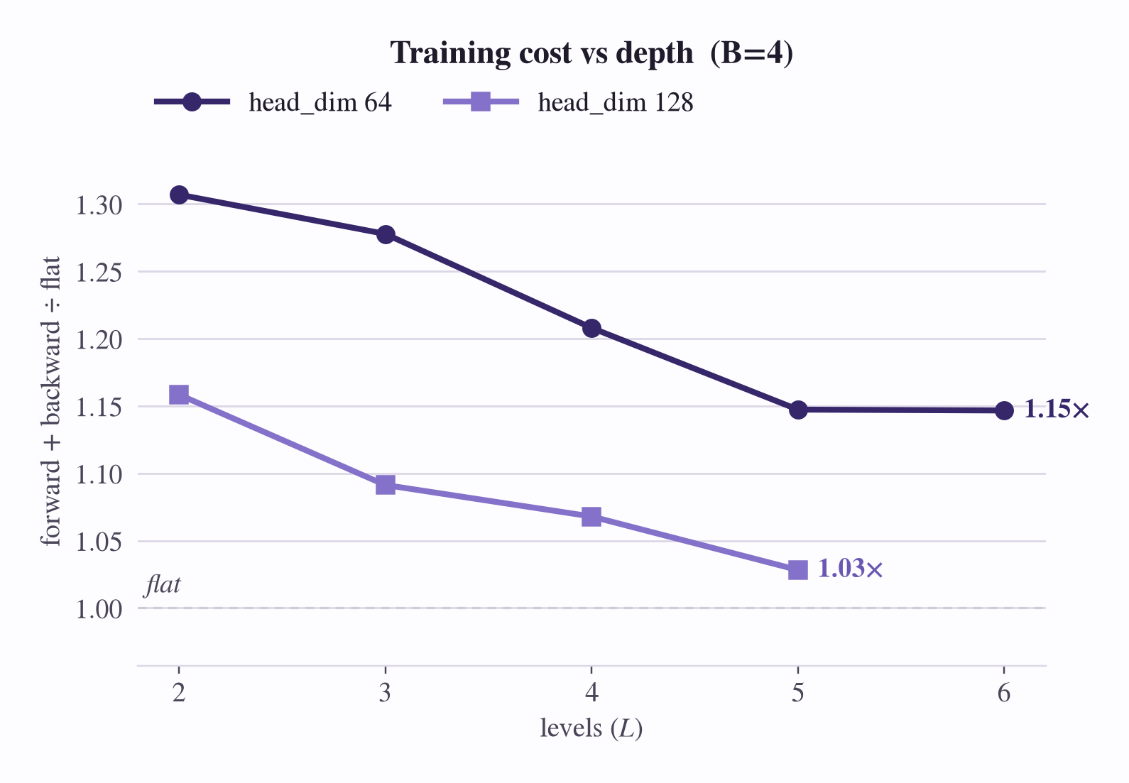
The nested forward is slower, 1.3–1.8× flat depending on batch size, and depth doesn’t help: at head_dim 64 it
sits around 1.4× from two levels through six. Nested just does more forward work per token. The backward is
where the hierarchy pays off. Upper levels lack the sequential structure that makes GDN-2’s backward
expensive, so adding a level is cheaper than adding the equivalent heads. On the combined pass, nested closes
on flat as depth grows (figure 1), reaching 1.03× at head_dim 128 with five levels.
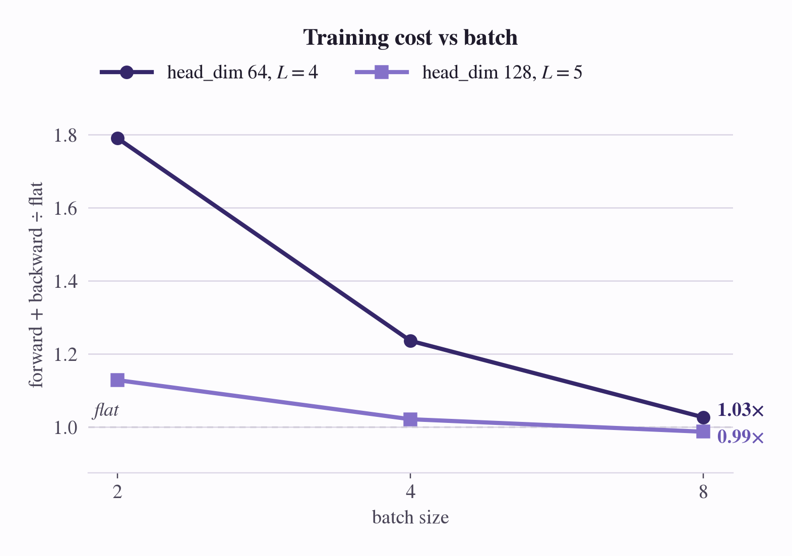
Batch size matters a lot at head_dim 64, which needs a big batch to keep the GPU busy, and barely at all at
head_dim 128 (figure 2). That’s convenient, because long sequences, where the hierarchy should help most, push
you toward small batches anyway.
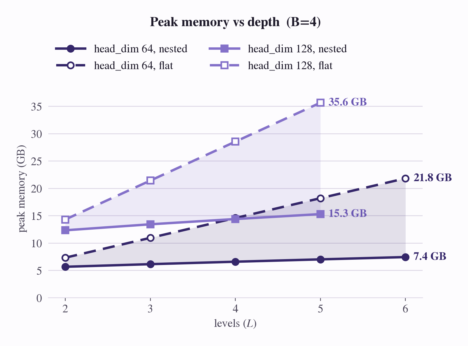
Memory is the clearest win (figure 3). Upper levels store one state per firing rather than one per chunk, so nested uses less memory than flat at every depth, and the gap widens with each level: about half of flat’s peak by four levels, a third by six.
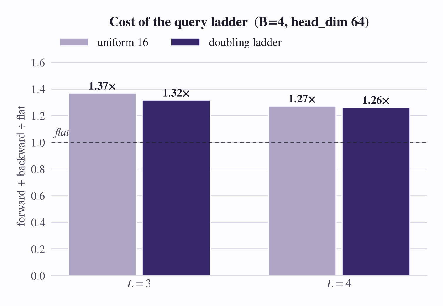
Finally, doubling queries per level costs essentially nothing next to a uniform 16 (figure 4).